Better Exploration for Symbolic Supervision

Despite the tremendous success that deep learning has shown in the past decade, there are certain application domains for which deep learning has traditionally been considered as not suitable. In particular, deep learning is notoriously known to be very data inefficient and to provide no guarantees with respect to the behaviour of the trained system. As a result of these limitations, the usage of neural networks in small data and safety critical domains has so far remained rather restricted. Nevertheless, there is a growing appetite among researchers to introduce neural networks to such domains as well. Our work explores one avenue to achieve this, namely to incorporate logic into deep learning.

The main strength of logic languages is their well defined semantics, making them suitable to represent knowledge and to facilitate formally correct, verifiable reasoning. Logic based systems are known to be very data efficient and provide all sorts of theoretical guarantees. Exactly what neural networks lack!

In particular, we consider scenarios where the learning supervision is provided wholly or in part by logical constraints, also referred to as “symbolic supervision”. Some of this comes from background knowledge: for example, we know a priori that humans are mammals and any prediction that claims that some human is not a mammal should be discarded. This way, even fully unlabelled samples carry some training signal, as the model prediction on such samples has to conform to the background knowledge. Another source of symbolic supervision is imperfect data collection: for example, in case human annotators cannot distinguish between different breeds of dogs, we may not know the exact label of a dog image, only that it comes from several of the possible breeds.

In this blog post, we explore two strongly related kinds of symbolic supervision: Disjunctive Supervision (DS) and Partial Label Learning (PLL). More details can be found in this paper: http://jmlr.org/papers/v25/23-0868.html.

Introduction

Partial Label Learning (PLL) deals with learning in the presence of imperfect supervision, where the training data has a set of labels, one of which is the true label. A scenario related to but different from PLL that we refer to as Disjunctive Supervision (DS) is when supervision gives multiple possible outputs and any one of these outputs is acceptable.

Note that there is no difference in the training data between PLL and DS. The formal difference concerns the assumptions about the underlying process, the corresponding task loss, and the evaluation methodology. For PLL, we assume an unknown joint distribution on the true function and on the noise model that generates the additional outputs. Its goal is, as in classical multi-class classification tasks, to learn the true value. In DS, however, we assume only an unknown process generating sets of labels. Our optimization problem is to maximize the expected value that the chosen output is one of the correct ones. Figure 1 summarizes the key differences.

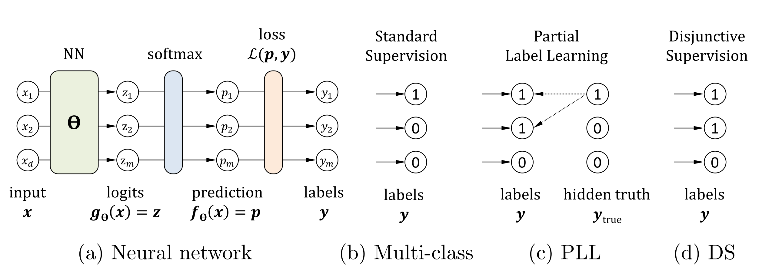
With multiple outputs labeled for a given input in the training set, supervision for PLL/DS also resembles supervision for multi-label classification. The key difference is that PLL/DS seek a function that produces a single output as the answer. Example 1 illustrates each task.

Example 1: Path Learning Scenarios

Consider a path finding problem in some dangerous environment: given endpoints A and B, we aim to find paths that take us safely from A to B. Standard multi-class learning is when there is a single safe path between A and B and it is provided for each training sample. In PLL too, there is a single safe path for each pair of endpoints, but it is not known for the training samples, only a set of paths that contains the single safe one. In multi-label learning, there are numerous safe paths and we aim to identify all of them. In DS, there are several safe paths and a valid model should identify one of them.

Formal Problem Statement

Supervised classification is the task of learning a function that conforms to a given set of samples
$D = {(x^{(j)}, y^{(j)})}_{j=1}^n$ where $\mathbf{x} \in \mathbb{R}^d$ is the input and $\mathbf{y} \in \{0, 1\}^m$ the one-hot encoded desired output (i.e. exactly one entry is 1). In Partial Label Learning (PLL) and Disjunctive Supervision (DS), however, there can be more than one allowed output, represented as $\mathbf{y}$ having multiple entries being $1$. The difference between PLL and DS is that the former assumes one single correct output among the given 1 entries that is unknown at training time, while the latter assumes that each of the entries are equally correct: thus the labels are not uncertain but “disjunctive”. We use $\mathbf{y}_{\text{true}}$ to denote the one-hot encoded unknown correct output, in the setting of PLL.

PLL assumes a joint data generating distribution $\mathbf{P}(x, y_{\text{true}}, y)$ on inputs $\mathbf{x} \in \mathbb{R}^d$, true one-hot outputs
$y_{\text{true}} \in \{0, 1\}^m$, and partial supervision $\mathbf{y} \in \{0, 1\}^m$.
In other words, the observed labels $\mathbf{y}$ are a distorted representation of the true labels $y_{\text{true}}$ and the former always includes the latter. The goal is to learn a function $\mathbf{f}$ in a given target class that maximizes

$$ \mathbb{E}_{P(x,y_{\text{true}},y)}\bigl[P\bigl(f(x)=y_{\text{true}}\bigr)\bigr] . $$

DS makes no assumption about a single true output $y_{\text{true}}$. It assumes only a joint data generating distribution $\mathbf{P}(x, y)$ on inputs $\mathbf{x}$ and partial supervision $\mathbf{y}$. Our target is to learn a function $\mathbf{f}$ that maximizes

$$ \mathbb{E}_{P(x,y)}\bigl[P\bigl(f(x)\in y\bigr)\bigr] . $$

As in supervised learning, we do not know the PLL/DS distribution $\mathbf{P}$: instead, we assume a finite
$D = {(x^{(j)}, y^{(j)})}_{j=1}^n$ sampled uniformly from $\mathbf{P}$ and we focus on optimizing performance on this set. Our learning target class will be a statistical model

$$\mathbf{p} = f_{\theta}(x) = \text{softmax}(g_{\theta}(x))$$

with input $\mathbf{x}$ and parameters $\theta \in \mathbb{R}^t$, interpreting its output as a probability distribution over the output space. The function $\mathbf{g}$ gives the unnormalized output, called logits, which we denote as $\mathbf{z}$.

Since the supervision is indistinguishable for PLL and DS (only its interpretation), technically, the same optimization methods are applicable, and most of our theoretical claims are relevant in both scenarios.

We aim to find the Maximum Likelihood Estimate (MLE), which maximizes the joint probability of the observed data. For DS, this means the probability, given $\mathbf{x}$, of observing an element $o$ such that $o \in \mathbf{y}$. While for PLL, it is the conditional probability given $\mathbf{x}$ of observing an $o$ with $o \in y_{\text{true}}$. For computational reasons, one usually minimizes the negative logarithm of this value:

Equation (PLL) cannot be optimized directly as $y_{\text{true}}$ is not known for training samples. In the absence of any prior preference over acceptable labels maximum likelihood methods use the candidate label set rather than the unknown label to define the likelihood, which corresponds to Equation (DS). This measure is known as the Negative Logarithm of the Likelihood function,
which yields the following sample-wise NLL-loss:

$$ \mathcal{L}_{\text{NLL}}(\mathbf{p},\mathbf{y}) = -\log\bigl(\mathbf{p}\cdot \mathbf{y}\bigr) = -\log\Bigl(\sum_{i=1}^{m}p_iy_i\Bigr) = -\log(P_{\text{acc}}) $$

The above formulation of the NLL-loss is a direct generalization of the classical case with a single allowed output to multiple allowed outputs and taking their probability mass together as
$P_{\text{acc}} = \sum_{i=1}^{m} p_i y_i$. The NLL-loss is a natural baseline for optimization; however, our paper shows that it is not an ideal choice for PLL/DS due to its sensitivity to initial configuration.

Main Results

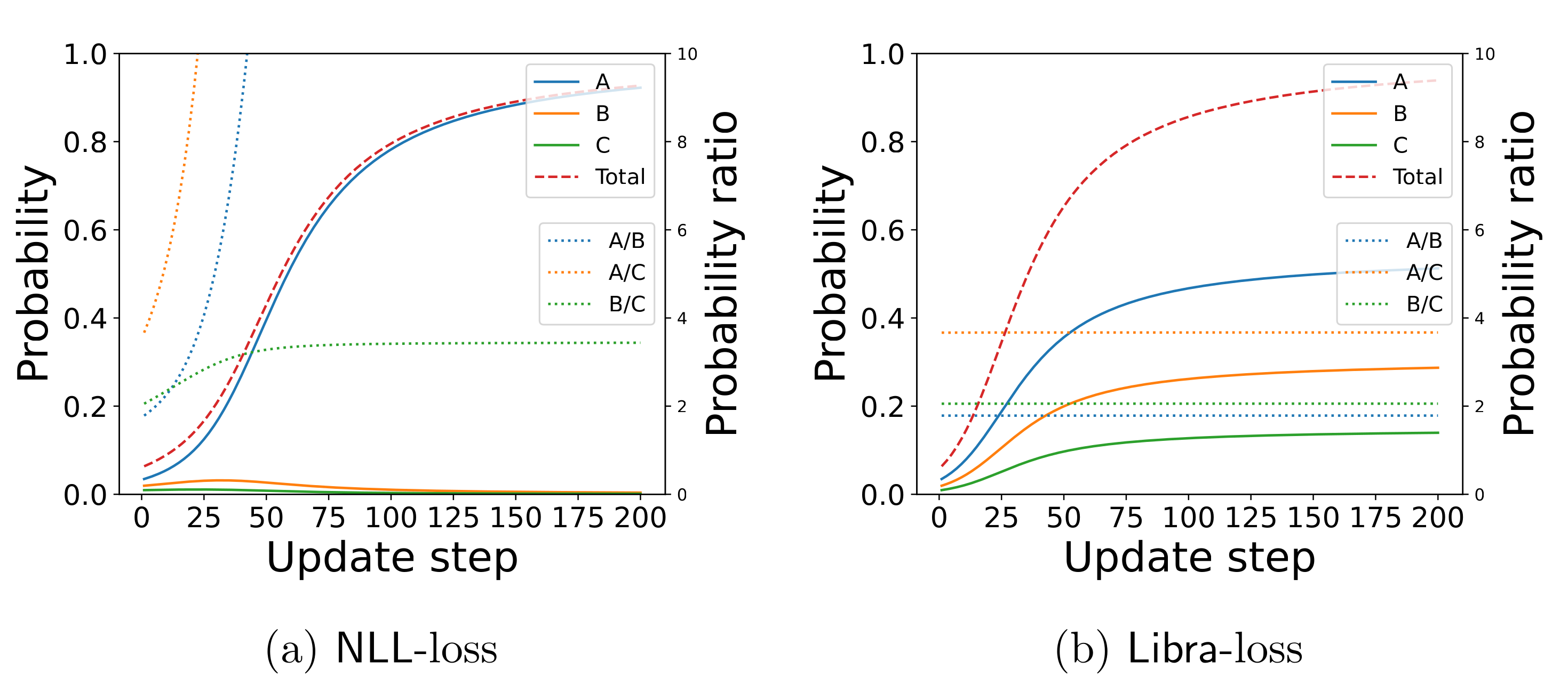
One important observation, described in the paper, is a bias phenomenon for architectures ending in a softmax layer when learning from partially-labelled datasets and using NLL-loss, which prevents proper exploration of alternatives. Due to this bias, the allowed output that has the highest probability at initialization ends up accummulating all the probability mass by the end of the training. We call this the winner-take-all phenomenon. To some extent, this result applies to several other popular losses from the literature.

The paper goes on to formulate a property to avoid the observed bias and derives from it the Libra-loss function, whose updates maintain the ratios of probabilities for acceptable labels produced by the softmax.

$$ \mathcal{L}_{\mathrm{Lib}}(\boldsymbol p, \boldsymbol y) = \underbrace{-\frac{1}{k} \sum_{i=1}^m y_i \log(\boldsymbol p_i)}_{\textbf{Allowed term}} + \underbrace{\log \bigg(1- \sum_{i=1}^m y_i \boldsymbol p_i \bigg)}_{\textbf{Disallowed term}} $$

where $k=\sum_i y_i$ is the number of allowed outputs. We show that when loss functions are restricted to depend only on the predicted probabilities of acceptable outputs, Libra-loss is uniquely defined (up to composition by differentiable functions). This more balanced loss leads to more stable training and increased success rate in finding a better optimum irrespective of the starting conditions.

Example 2

Let us examine a toy problem with 10 inputs and m = 100 outputs. We assume a single training sample (x, {A, B, C}), i.e., having $k=3$ allowed outputs. We train a neural network that consists of a single dense layer with 100 neurons and softmax non-linearity, having 1100 parameters altogether. Figure 2 shows the behavior of the standard NLL-loss and our Libra-loss, both starting from the same initial condition. NLL-loss results in a distribution where the allowed output A with the highest initial probability accumulates all the probability mass. In contrast, Libra-loss yields a balanced update and the ratio of the allowed outputs does not change.

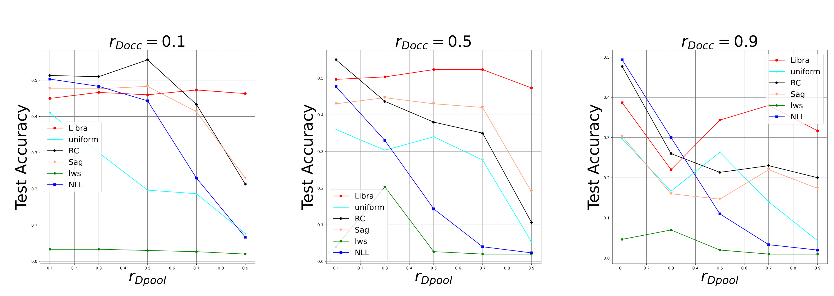
The paper compares several methods from the PLL literature experimentally both on synthetic and real-world datasets. We find that Libra-loss is more robust than other variants when the learning task becomes harder, either because there are more labels in the label sets or because some distractor labels co-occur very often with the true label. To illustrate this, let us look at one of the experiments from the paper.

This experiment is based on the CIFAR-100 dataset, which has 100 labels. We add synthetic disjunctive noise, controlling the number of distractors (r_Dpool) and the strength of distraction (r_Docc).
Figure 3 shows that performance degrades as r_Dpool (number of distractors) and r_Docc (strength of distraction) increase. However, Libra-loss shows remarkable robustness.

Conclusion

We identify a bias phenomenon that emerges in Partial Label Learning based on neural architectures with a softmax layer. We provide a loss function which is tailored towards addressing the situation, and argue that it is, up to a differentiable transformation, canonical. We also give an experimental evaluation of its performance.